This page presents some formation control experiments, made during the Submeeting event, between the 27th and the 31th of May 2024, at Saint-Raphaël in the south-east of France. In these experiments, two ROVs from ENSTA Bretagne were controlled to reach a triangular formation as illustrated by Figure 1.
I – Experimental setup
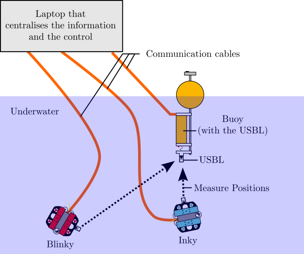
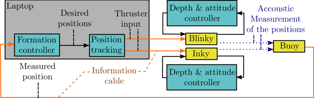
Figure 2 gives an overview of the experimental setup. The two ROVs Inky and Blinky are connected by cable to the same laptop computer that centralises the control and the information. The laptop is also connected to a buoy equipped which can localise the robots with an Ultra Short Baseline (USBL) acoustic sensor.
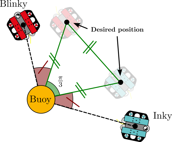
of the equilateral triangle.
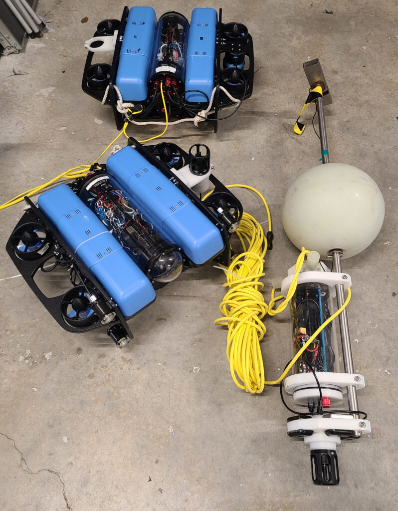
The ROVs, depicted in Figures 3 and 4 are BlueROV2 from the BlueRobotics company. These low-cost commercial robots are very common in the academic field and are well-documented online. They have the same thruster configuration, called ‘heavy’, with 8 thrusters that control their 6 degrees of freedom. They are equipped with:
- a Raspberry Pi 4 Computer.
- a frontal monocular camera used to record videos of the experiment.
- a barometer used to measure the robots’ depth.
- an IMU to measure their orientation and their heading but it is not accurate enough to provide forward speed. The robots’ IMUs are used in the ROVs’ attitude control, but not in their position control.
- a X150 micro-USBL beacon from the Blueprint Subsea company. This model of USBL has a delay of a minimum 4s between two measurements.
A dynamical model of the BlueROV as well as some control advice are presented in [1]. The robots are programmed along with the ROS2 middleware. Moreover, they have translation and rotation commands provided by the MAVROS package. The thrusters produce a maximum translation thrust of about 80 N, which allows
the vehicle to reach a maximum horizontal velocity of about 1.5m/s. Forward and lateral inputs must be provided in PWM whose value is between 1000 and 2000, where 1500 is the neutral input, and 1000 and 2000 are the maximum power in one direction or the other. However, the motors have a dead band such that they are inactive if one input is in the interval [1450, 1550]. The USBL buoy, also depicted in Figure 3 is a prototype that was designed at the ENSTA Bretagne to localise the two robots. It is equipped with an X150 micro-USBL beacon and a Razor IMU. The USBL is configured to send ping to the USBL beacon of the ROVs, to measure their position in its own frame. The IMU allows transforming the robot’s position into the North-oriented global frame.
The centralised formation control
The formation control is described in Figure 5. The laptop centralises the control. From the measured horizontal positions of Inky and Blinky, the desired positions of the ROVs are computed with the formation controller. Then, a position-tracking controller computes the thruster setpoint sent to Inky and Blinky. In parallel, the depth and attitude of the ROVs are controlled by an independent decoupled controller. Finally, the Buoy uses its USBL and IMU to measure the position of the two ROVs. Note that the ROVs do not communicate or see each other to control their position.
Experimental protocol
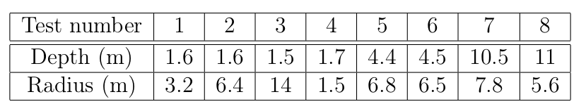
Protocol to evaluate the precision of the localisation. To evaluate the period and the precision of the USBL, 8 tests were conducted. One ROV was in the water, with a fixed position, which was measured. From the measurement of this fixed position, the standard deviation of the period and the measurement can be computed to evaluate the precision. Two different environments were tested: the shallow water and the sea. The depth and the radius of the ROVs during these tests are given by Table 1. Tests 1,2,3 and 4 were conducted in shallow water, next to the pontoons of the Port de Boulouris. Blinky was placed on the seabed at different distances from the buoy and had a fixed position. The buoy was sheltered from the swell. Since the USBL is in shallow water, there were a lot of acoustic disturbances. Tests 5,6,7 and 8 were conducted at sea next to Le Lion de Mer at Saint-Raphael. Inky was controlled to stay at a fixed depth. The horizontal position was not controlled and was assumed constant. The buoy oscillated with the swell. Since the USBL is at sea, there were fewer acoustic disturbances.
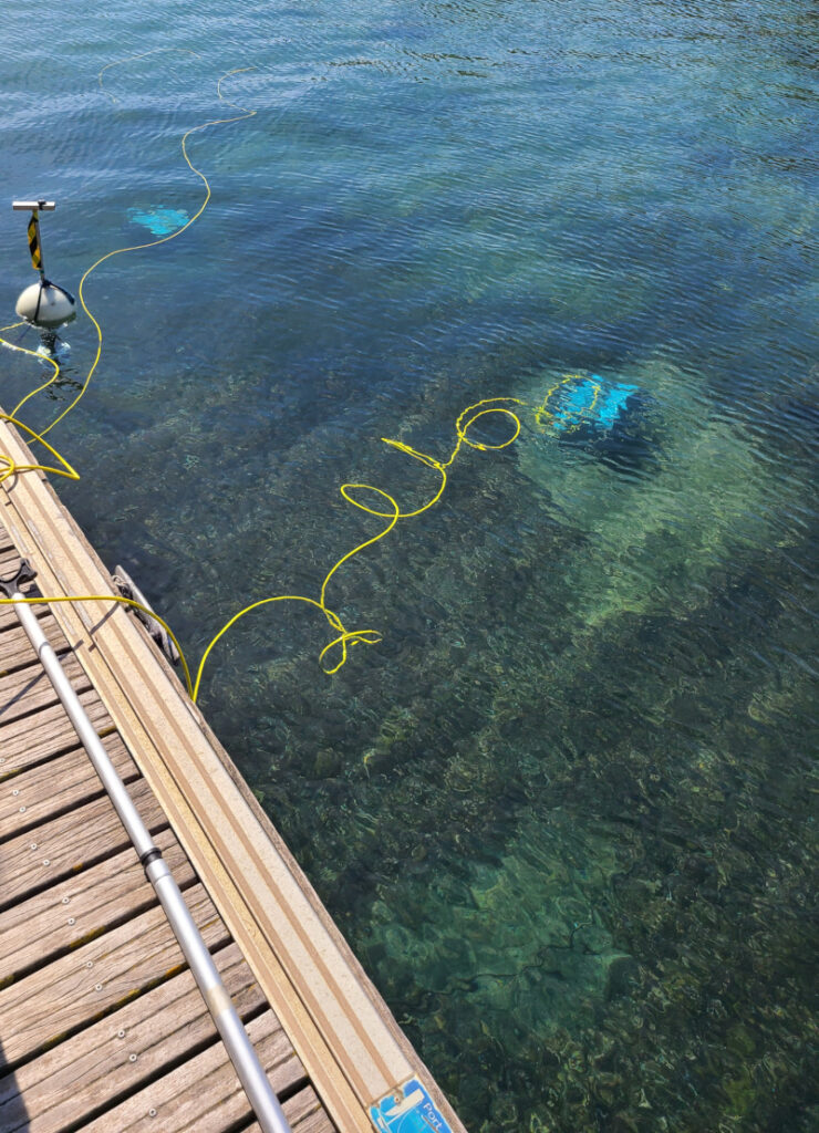
Formation control protocol. The formation control with two ROVs was tested with the minimum USBL delay (≃ 4s between two measurements), in different configurations. Test 12 is a formation control conducted in shallow water, at the same place as tests 1 to 4 with the same weather conditions, illustrated by Figure 4. Tests 9 to 11 are formation control conducted at sea right after tests 5 to 8.
Protocol to test the limit of stability. In addition, to test the limit of the stability of the system with respect to delays, an additional delay δt was added between the USBL measurement at time t and the use of this measurement by the controller at time t+δt. This artificial delay can simulate a filtering delay in the USBL measurement, which would be required if the acoustic signal were to deteriorate. In theory, when the delays increase, the controller uses older information, and so the stability of the system decreases. However, the measurement period stayed the same. This delay was applied to the tests 13 to 15. The additional delay is 1 s for test 13,2s for test 14 and 4s for test 15. Tests 13 to 15 were conducted in shallow water, right after test 12.
II – Results
The quality of the localisation
As presented earlier, tests 1 to 8 were conducted to evaluate the quality of localisation. In this section, the quality is evaluated by computing standard deviations
for the USBL measurement period and the measured ROV position.
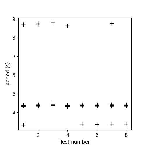
Measurement period Figure 6 presents an evaluation of the USBL measurement period T for the tests 1 to 8, where only one ROV is localised. There is a marker for each measured period. There is 3% of outliers. Some outliers correspond to 2·T when a measurement is missed because the USBL is not able to receive the response from the ROV. Without the outliers, the mean period is T = 4.37s with a standard deviation of σT = 0.03s.
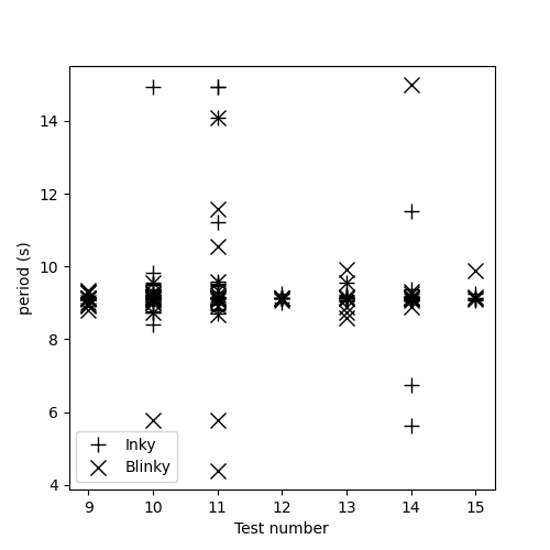
Figure 7 presents the same evaluation for tests 9 to 15, where two ROVs are localised. There is 7% of outliers. Without the outliers, the mean period is T = 9.14s with a standard deviation of σT = 0.17s. As expected, with two ROVs in the water, the USBL must alternate the measurements, so the period is twice as long. Moreover, with two ROVs, the measurements are less regular. Nevertheless, the standard deviation is slow enough to assume a constant measurement period.
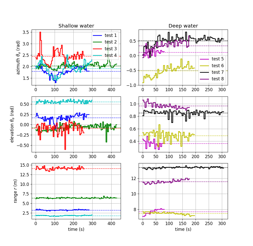
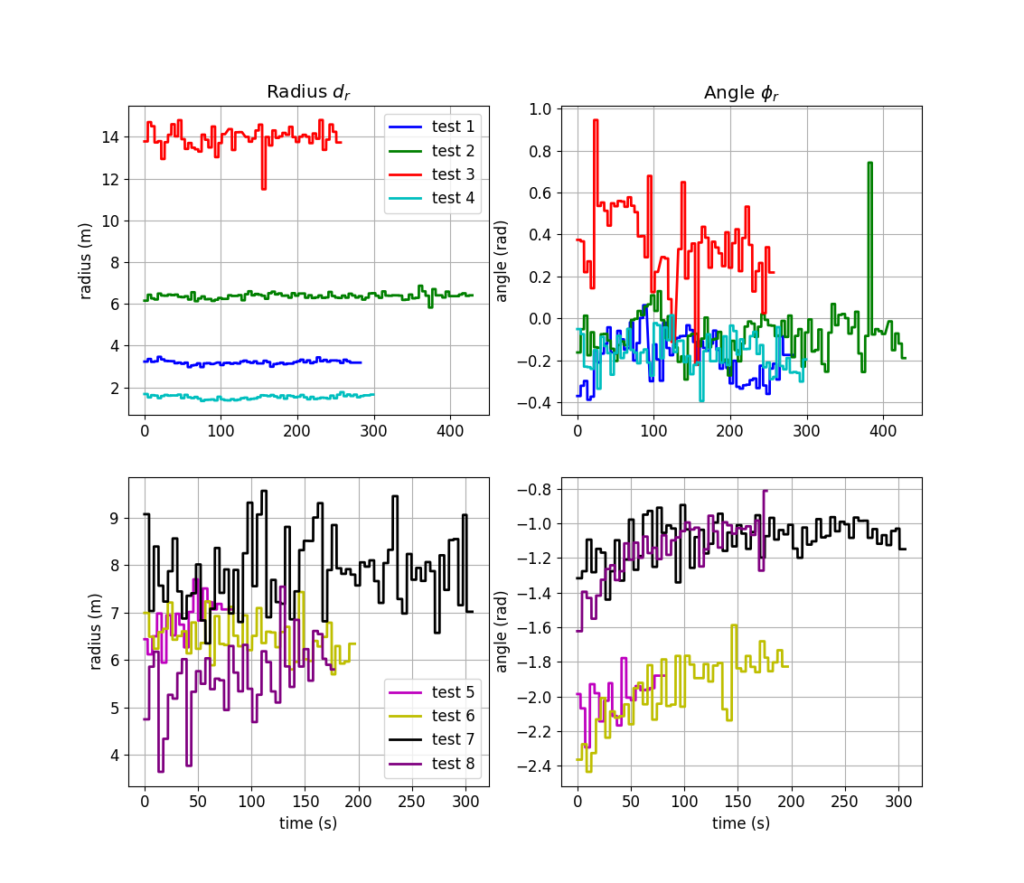
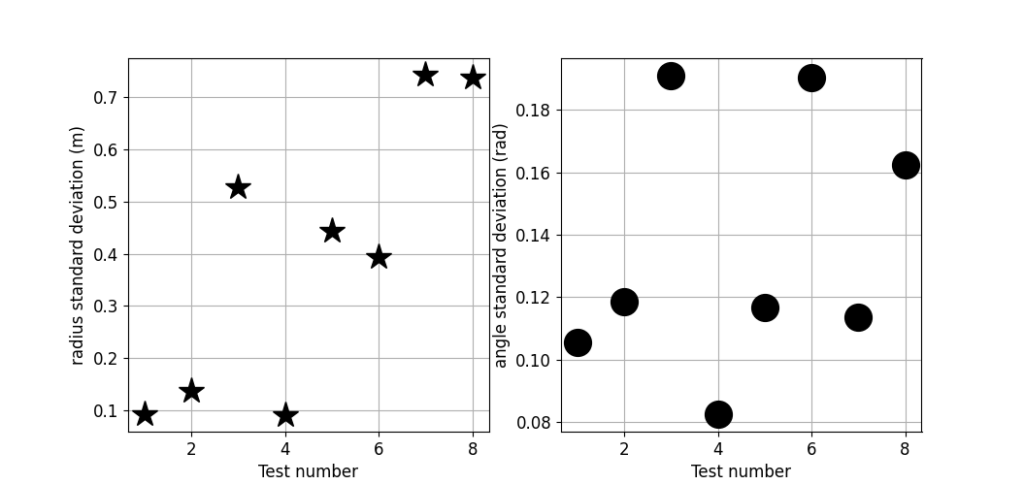
Position measurement The USBL measurements are displayed on Figure 9, the IMU measurements are displayed on Figure 8, the estimations of the ROV polar coordinates (dr, ϕr) are displayed on Figure 10 and the standard deviation of the localisation (σd , σϕ ) is displayed on Figure 11. Since the position of the ROV is
assumed fixed, the oscillations in Figure 10 are considered estimation errors.
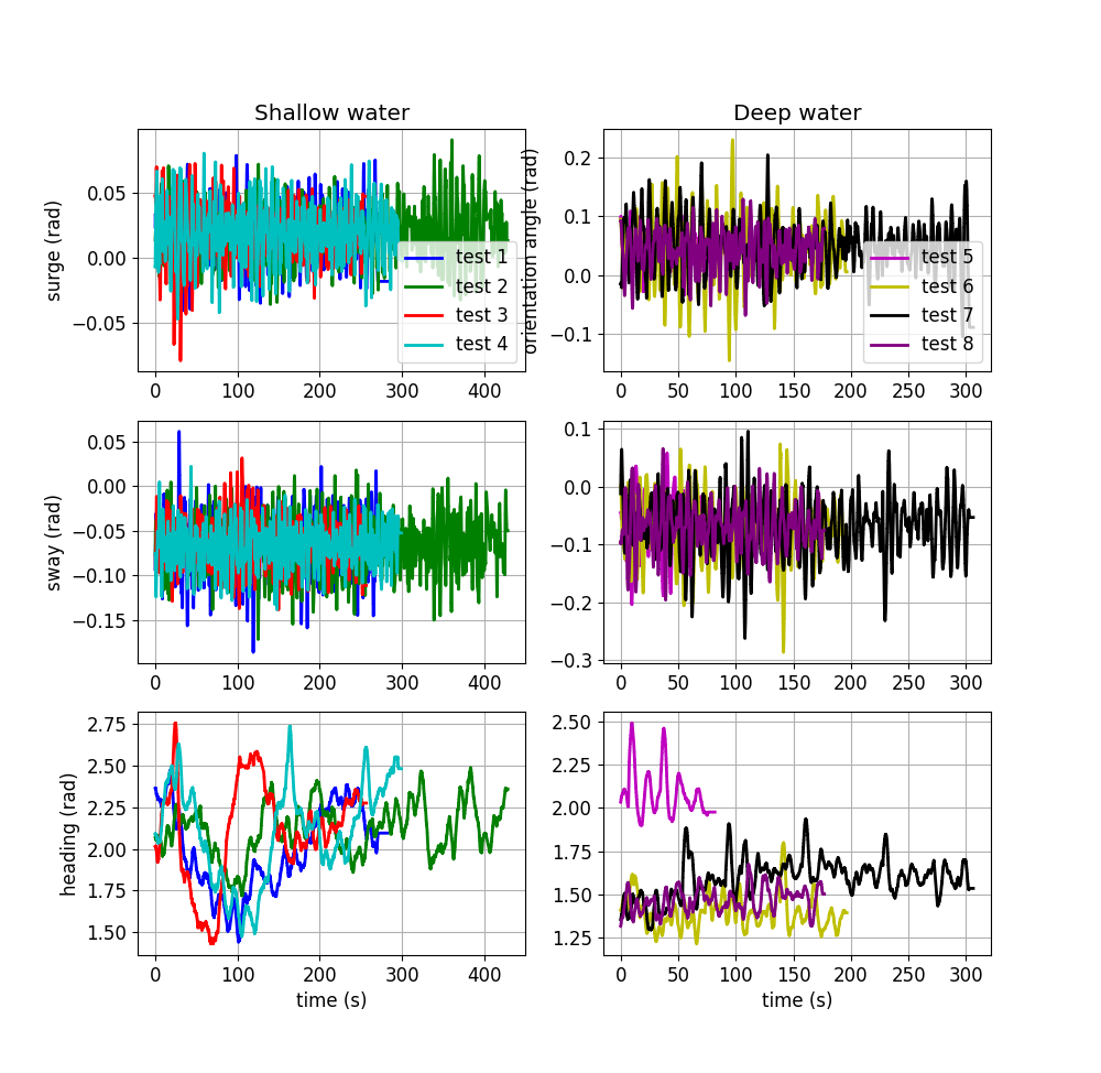
As visible in Figure 8, the sway and the surge of the buoy oscillate with the swell. The amplitude is about 0.05 rad in shallow water (tests 1 to 4) and 0.1 rad at sea (tests 5 to 8). Thus, the swell is more important at sea. Moreover, the heading of the buoy changes over time in a range of ±0.5 rad. Therefore, it is important to compensate for the buoy motion in the localisation of the ROV.
In addition, on Figure 11, the radius dr is more precise in shallow water, for the tests 1,2 and 4 (σ < 0.2 m), except for the test 3 (σd ≃ 0.52 m). Moreover, at sea, σd is higher for the deep tests 7 and 8 (σd > 0.7 m) compared to the less deep tests 5 and 6. Regarding the angle ϕr, the standard deviation is higher for the tests 3, 7 and 8 (σd > 0.16 rad) compared to the other tests (σd < 0.12 rad). All these differences can be explained as follows.
The test 3 is the worst configuration for the USBL, acoustically speaking. In the test 1 to 4, the ROV is in shallow water, at a depth of about 1.5 m. The motion of the
buoy is similar for these four tests, as illustrated by Figure 8. While for tests 1,2 and 4, the ROV is under a radius of 7 m, the radius is about 14 m for test 3. As a result, there are more acoustic disturbances for test 3. Due to the shallow water, there are more reflections of the acoustic signal between the surface and the seafloor. These reflections create more acoustic multi-path which reduces the precision of the USBL measurement. Thus the quality of the USBL measurement is deteriorated for test 3, as illustrated by Figure 9. For the tests 1,2 and 4, the standard deviation of θ e is about 0.07 rad and the standard deviation of the range r is about 0.1 m. However, for test 3, their standard deviations are respectively 0.13 rad and 0.3 m. In practice, although the X150 micro-USBL is presented as omnidirectional on the datasheet of the manufacturer, the USBL localisation is often accurate when robots are inside a cone under the buoy. The omnidirectionality of the USBL has not been tested. For test 3, the ROV is too probably far from this cone to be detected accurately.
Moreover, the measurement of the buoy’s IMU and the buoy’s USBL were not precisely synchronised. As a result, when the buoy oscillates with the swell, the
amplitude of the localisation error is increased. In Figure 8, the buoy oscillates more at sea than in shallow water. This can explain why the sea tests (5 to 8) have a higher σs , even though there is less acoustic disturbance at sea. Furthermore, this synchronisation error creates an error of angle, so the radius error is proportional
to the radius. This is why σ d is higher for tests 7 and 8 at a depth of about 10 m compared to the test 5 and 6 at a depth of about 5 m. Because of this synchronisation error, the localisation is not reliable in heavy swell.
In addition, on Figure 10, for the tests 6 and 8, the angle ϕr drifts. The ROV probably moved during these two tests. So the value of σ ϕ is not relevant for tests 6 and 8.
As a result, the error of precision of the localisation of the ROV is non-neglectable and has some impact on the formation control. From Figure 9.12, the standard
deviation of the radius dr and the angle ϕr can be evaluated as

The quality of the formation control
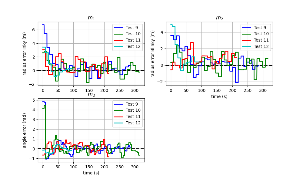
From the data of the experiments, it is possible to display the discrete state vector

The state of the system is expected to converge in a neighbourhood of the equilibrium point, whose size is of the same order as σd for m1,j and m2,j and the same order as 2·σϕ for m3,k. Figure 12 presents the time evolution of mj for the tests 9, 10, 11 and 12. During these tests, the system was stable and the ROVs converged towards a neighbourhood of the equilibrium point. The size of the neighbourhood is visually coherent with the standard deviation of the ROV localisation. In this neighbourhood, the ROVs can see each other as illustrated by Figure 5.
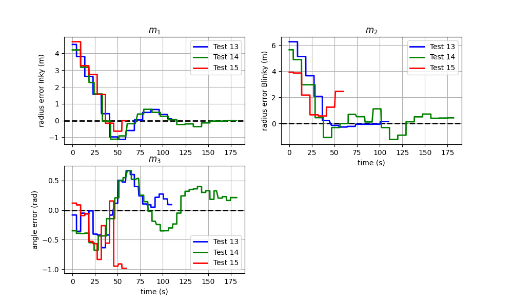
Deterioration of the stability with additional delays. Figure 13 presents the time evolution of mj for the tests 13, 14 and 15, where a delay δt is added in the USBL measurement. the USBL measurement at time t is used by the controller at time t + δt. The additional delay is 1 s for test 13, 2 s for test 14 and 4 s for test 15. One can observe that the formation converges to a stable neighbourhood with 1s and 2s of additional delays. However, the state m 3 starts to diverge for the test 15 with 4s of delay, hence the premature stop of this test. During test 15, the ROVs spun around the buoy, one ROV was fleeing, and the second ROV was chasing the
first.
III – Discussion
Following the results, the triangular formation control with two ROVs is achieved with two ROVs. The control is stable in the sense that the robots converge in a neighbourhood of the equilibrium point. The size of this neighbourhood is coherent with the precision of the localisation.
The acoustic localisation is harder to achieve for a large number of robots. The USBL of the experiments locates only one robot at a time with a ping. Thus, the USBL measurement period proportionally increases with the number of robots (+4 s per robot). Sending pings to different robots at the same time can reduce the period, but the precision of the localisation is deteriorated by ping interference. An alternative is to synchronise the buoy and the robots with the same clock, so that the buoy simply listens to the acoustic messages sent by the robots, knowing in advance the time of their transmission. But it’s not easy to synchronise all the robots.
Moreover, the ground truth was not recorded during the experiments. Future experiments should compare the discrete-time measured positions with the real con-
tinuous-time positions of the robots in order to show that the continuous part of the system is also stable. However, to record the real position of the robots, one needs a high-precision and high-frequency measurement of the position, which is difficult to implement in an outdoor environment.
In addition, the localisation precision deteriorated because the buoy’s IMU and USBL were not precisely synchronised. As the buoy moves with the swell, it creates
some error in the computation of the position in the world frame. However, if the IMU and the USBL are precisely synchronised, the localisation is not deteriorated by
the buoy’s movements, especially when the robots are far from the buoy.
Finally, as expected, adding delays in the control loop decreases the stability of the formation control. Therefore, delays must be considered in the stability analysis,
when they are significant, to know what is the maximum delay the system can have while remaining stable.
Bibliography
[1] Tor Harald Staurnes, Pål Kristoffer Kjærem, Lauritz Rismark Fosso, and Kristian Aasmundstad Johannesen. Decentralized Model Predictive Control for Increased Autonomy in Fleets of ROVs. Bachelor thesis, NTNU, 2023. Accepted:2023-07-12T17:21:26Z.